


About a decade ago, I wrote two articles:
- Modulation Alternatives for the Software Engineer (November 2011)
- Isolated Sigma-Delta Modulators, Rah Rah Rah! (April 2013)
Each of these are about delta-sigma modulation, but they’re short and sweet, and not very in-depth. And the 2013 article was really more about analog-to-digital converters. So we’re going to revisit the subject, this time with a lot more technical depth — in fact, I’ve had to split this article into three parts — and a focus on the digital-to-analog conversion side. The DAC case is interesting because all we’re doing is creating a series of low/high pulses at each clock tick, then putting them through a simple linear filter. There are very few opportunities for the introduction of unmodeled dynamics or sources of error, so we should expect very close results to any simulation.
We’ll be covering a number of aspects of first-order and second-order delta-sigma modulators, with roughly the following outline:
- Part 1: Basics of modulation: kernels, block diagrams, linear analysis, choice of coefficients, and frequency spectra
- Part 2: Filtering tradeoffs, error analysis, and effects of low duty cycles
- Part 3: Implementation issues, including integer math and accumulator ranges
I’ll be using some theory, but you can learn a lot from empirical investigation; we’ll do the usual messing around in Python and see what we can find out.
Oh — and there’s one teensy little practical snag we’ll have to deal with. Please read all three parts, because I won’t bring it up until the discussion of implementation issues, and if you build a system based on the content of Part 1 or Part 2, you’re likely to run into this and it will ruin your day.
For now, though, let’s just keep it simple.
Author’s Note: I originally wrote this series of articles in January and February 2019, but put them on hold for various reasons. At the time, Parts 1 and 2 were essentially complete, and Part 3 was unfinished. I will try to publish Part 2 and Part 3 in a timely fashion, but it may take a while, so if you are reading this, please be patient.
Also a note about terminology: both “sigma-delta” and “delta-sigma” are used in practice, and mean the same thing, but “delta-sigma” seems to have the broader use. (See for example recent content from Texas Instruments and Analog Devices, and various books.)
Anyway: here we go!
First-Order Delta-Sigma
Let’s start out with a Python implementation of the algorithm I mentioned in 2011, which has the following “kernel” to process an output \( y[k] \) from an input \( x[k] \) that is between 0 and 1:
accum1[k] = accum1[k-1] + R*(x[k] - A*y[k-1])
y[k] = 1 if accum1[k] >= R*A else 0
I’m going to use the numpy and scipy and matplotlib packages.
%matplotlib inline
import numpy as np
import matplotlib.pyplot as plt
import matplotlib.gridspec as gridspec
import matplotlib.ticker as ticker
import matplotlib
import scipy.signal

matplotlib.rcParams['mathtext.fontset']='cm'
def dsmod1(x, A, R=1, modulate=True):
    """ first-order delta-sigma modulation """
    y = np.zeros_like(x)
    n = len(y)
    accum = 0
    out = 0
    M = 1 if modulate else 0
    for i in range(n):
        accum += R*(x[i] - out*A)
        out_q = 1 if accum >= R*A else 0
        out = (M*out_q
              +(1-M)*accum)
        y[i] = out
    return y
dsmod1.argformat = ''

def samplewave(T=1,dt=0.002):
    t = np.arange(0,T+1e-5,dt)
    x = 1-np.abs(4*t-1)
    x[4*t>2] = 0.95
    x[t>0.75] = 0.02
    return t,x

def describe_dsmod(dsmod, args):
    sdtype = dsmod.__doc__.splitlines()[0].strip()
    try:
        sdargfmt = dsmod.argformat
    except:
        sdargfmt = ''
    return sdtype + sdargfmt.format(*args)

def show_dsmod_samplewave(t,x,dsmod,args=(1,),tau=0.05, R=1, fig=None,
                          return_handles=False, filter_dsmod=False):
    dt = t[1]-t[0]
    if filter_dsmod:
        x1 = dsmod(x, *args,R=R, modulate=False)
    else:
        x1 = x
    y = dsmod(x,*args,R=R)
    a = dt/tau
    yfilt = scipy.signal.lfilter([a],[1,a-1],y)
    xfilt = scipy.signal.lfilter([a],[1,a-1],x1)

    if fig is None:
        fig = plt.figure(figsize=(10,7), facecolor='white')
    gs = gridspec.GridSpec(3, 1,height_ratios=[2,0.4,1])
    axes = [fig.add_subplot(gs[k]) for k in range(3)]
    ax0 = axes[0]
    ax0.plot(t,x,label='x(t)')
    ax0.plot(t,yfilt,label='LPF(y(t))')
    ax0.plot(t,xfilt,label='LPF(x(t))')
    ax0.legend(labelspacing=0,loc='upper right',fontsize=10)
    ax0.set_ylabel('x, LPF(x), LPF(y)')
    ax0.set_xticklabels([])

    ax1 = axes[1]
    ax1.step(t,y,linewidth=0.5)
    ax1.set_ylim([-0.1,1.1])
    ax1.set_yticks([0,1])
    ax1.set_ylabel('y')
    ax1.set_xticklabels([])

    ax2 = axes[2]
    filt_error = xfilt-yfilt
    ylim = (min(filt_error),max(filt_error))
    # plot margin
    s = 0.08
    ylim = (ylim[0]*(1+s)-ylim[1]*s, ylim[1]*(1+s)-ylim[0]*s)
    ax2.plot(t,filt_error)
    ax2.set_ylim(ylim)
    for s in [-1,1]:
        # approximate error bounds; we'll show why later in the article
        ax2.plot([t[0],t[-1]],[s*a/2,s*a/2],color='#008000',linewidth=0.8,dashes=[8,8])
    ax2.set_ylabel('error')
    ax2.get_yaxis().set_major_locator(ticker.MaxNLocator(12,steps=[1,2,5,10]))
    ax2.set_xlabel('time (s)')
    ax2.grid(True,linestyle=':')

    for ax in axes:
        ax.set_xlim(min(t),max(t))

    fig.subplots_adjust(hspace=0.1)
    fig.suptitle('Delta-sigma modulation (%s)\nwith RC filter $\\tau=%.2f s = %.1f\\Delta t, R=%.2f$'
                 % (describe_dsmod(dsmod,args), tau, tau/dt, R))
    if return_handles:
        return fig, (ax0,ax1,ax2)

t,x = samplewave()
show_dsmod_samplewave(t,x,dsmod1,filter_dsmod=True)
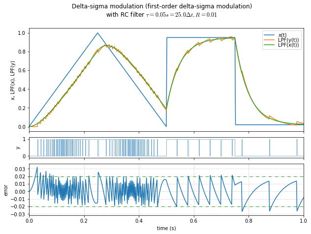
Now, there is an amazing amount of information we can see in the graph above, from just a handful of lines of Python. What are we looking at?
The top subplot contains \( x(t) \), a sample waveform that starts with a triangle wave and ends with a square wave. We feed this into our 1st-order delta-sigma modulator and we get out a pulse train \( y(t) \) in the middle subplot, which sort of looks like a PWM waveform except that it isn’t constant frequency. We have an accumulator, and whenever it gets to some threshold \( R\times A \), we output a 1, and next time we subtract \( R\times A \) from the accumulator; otherwise we output a zero.
The DC gain from input to output is \( 1/A \). If you have floating-point data limited between 0 and 1, use \( A=1 \). This will produce unity gain at low frequencies; since we’re integrating \( x(t)-Ay(t) \), if \( A=1 \) then the low-frequency components of \( x(t) \) and \( y(t) \) balance each other out. If you have fixed-point integer data limited between 0 and some value \( A \), use that \( A \) instead.
The fun comes when we filter the input \( x(t) \) and the output \( y(t) \) with a first-order low-pass filter. The results are shown in the top subplot, and they follow each other very well, because at low frequencies \( x(t) \) and \( y(t) \) are essentially identical. The error between the filtered waveforms is shown in the bottom subplot, and it’s essentially limited to a small band that turns out to be limited to approximately \( \pm\Delta t/2\tau \) for smoothly-changing inputs, as we’ll see later. (In this case, \( \Delta t = 0.002 \)s and \( \tau=0.05 \)s, so the theoretical value of error band amplitude is \( \pm0.02 \), which matches our example waveform fairly well.)
This is a very simple DAC; we implement our delta-sigma modulator digitally, and take our pulse waveform and feed it through an RC filter.
Linear Analysis of 1st-order Delta-Sigma Modulation
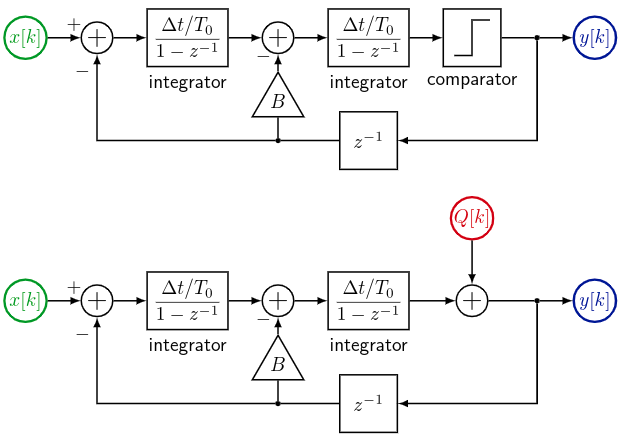
The modulator itself is usually analyzed with a linear approximation for the threshold comparator, namely that we replace it with an additive noise waveform \( Q(t) \), or \( Q[k] \) for discrete-time analysis, that is uncorrelated with anything else. (There are only two ways we can get away with this. One is if the integrator output is zooming around so much that the difference between the integrator output and the modulator output looks enough like noise. This happens if the input frequency spectrum is “interesting” enough, or in certain cases of “uninteresting” input, like DC inputs where the DC level is not near 0 or 1. The second possibility is if we add an intentional “dither” noise signal to the threshold comparator input, improving the validity of this noise approximation, at the expense of additional output noise.)
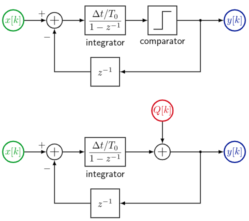
Here \( \Delta t \) is the timestep for the discrete-time system; \( T_0 = \Delta t / R \) is a tunable integrator parameter, but it’s pretty standard to use \( T_0 = \Delta t \) so that \( R = \Delta t/T_0 = 1. \)
The transfer function from input \( x(t) \) to output \( y(t) \) is \( H(z) = R/(1-z^{-1})/(1+Rz^{-1}/(1-z^{-1})) = \dfrac{R}{1+Rz^{-1} - z^{-1}} \) which has a pole at \( z=1-R \), and is therefore stable for \( 0 < R < 2 \), with marginal stability when \( 0 < R \ll 1. \) The noise transfer function from quantization noise \( Q(t) \) to output \( y(t) \) is \( N(z) = 1/(1+Rz^{-1}/(1-z^{-1})) = \dfrac{1-z^{-1}}{1+(R-1)z^{-1}} \).
Let’s graph these for a few values of \( R \):
fig = plt.figure(figsize=(8,6), facecolor='white')
ax = fig.add_subplot(1,1,1)
f = np.arange(0,0.5,0.001)
# frequency, normalized to 1/delta T
for R in [0.1,0.5,1.0,1.5]:
    z = np.exp(2j*np.pi*f)
    zinv = 1/z
    H = R/(1+(R-1)*zinv)
    N = (1-zinv)/(1+(R-1)*zinv)
    line = ax.plot(f,np.abs(H), label='$H(z), R=%.1f$' % R)
    linecolor = line[0].get_color()
    ax.plot(f,np.abs(N),color=linecolor,linestyle='--',
            label='$N(z), R=%.1f$' % R)
    x0 = 0.5
    ax.plot([0,x0],[0,x0*(2*np.pi/R)],'-',color=linecolor,linewidth=0.4)
ax.legend(labelspacing=0, fontsize=12, loc='upper left')
ax.set_xlabel('$f\Delta t$', fontsize=16)
ax.set_xlim(0,0.5)
ax.set_ylabel('$|H(z)|, |N(z)|$', fontsize=16)
ax.set_ylim(0,4.1);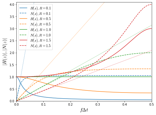
This shows that \( H(z) \) is a filter with unity gain at low frequencies — for \( R<1 \) it is a low-pass filter; for \( R>1 \) the gain actually increases. On the other hand, its complement \( N(z) \) suppresses frequency content at low frequencies, where \( N(z) \approx 2\pi f\Delta t/R \). This is the intended effect; we want the remaining noise energy to be in the higher frequency ranges so that a low-pass-filter on the output will get rid of most of it.
(I should note in passing that I dislike using z-transform analysis, mostly because of my lack of familiarity. It’s very useful, but I find it a lot less intuitive than Laplace (s) domain analysis, so sometimes I just pretend that a system is continuous-time and use s-domain analysis instead. This works okay as long as the frequency content is small once it gets to near Nyquist frequency \( f_s/2 \), otherwise you need z-transforms to stay accurate.)
With linear analysis, it looks like the value of \( R \) could be increased to help attenuate quantization noise further. Unfortunately, this is not actually the case; the assumption of uncorrelated noise breaks down. We can try looking at the effect of changing the integrator gain \( R \) in a test simulation of a delta-sigma modulator, but it doesn’t change the behavior at all. This seems really weird, until you look more closely at the kernel equations:
accum1[k] = accum1[k-1] + R*(x[k] - A*y[k-1])
y[k] = 1 if accum1[k] >= R*A else 0
We can make the substitution accum1[k] = R*acc_n[k], at which point we have
acc_n[k] = acc_n[k-1] + x[k] - A*y[k-1]
y[k] = 1 if acc_n[k] >= A else 0
This is the same behavior, independent of \( R \), so all that a change of \( R \) is doing is to change the scaling of the integrator value relative to input \( x \) and output \( y \).
Below are two other graphs with \( R=0.01 \) and \( R=100.0 \).
t,x = samplewave()
show_dsmod_samplewave(t,x,dsmod1,R=0.01)
t,x = samplewave()
show_dsmod_samplewave(t,x,dsmod1,R=100.0)

See? Changing \( R \) doesn’t make any difference. So we’ll just use \( R=1 \) from here onward.
Frequency Spectrum of 1st-order Delta-Sigma Modulation
Let’s get a little more sophisticated and measure the frequency spectra of the modulated output from a couple of input waveforms \( x(a_0,a_1,t) = a_0 + a_1 \sin \omega_1 t, \) which is just a sine-wave plus a DC offset.
def enumerate_reverse(somelist):
n = len(somelist)
while n > 0:
n -= 1
yield n, somelist[n]
def f1_noise(t,a0,a1):
r = np.random.RandomState(seed=123)
return (r.randint(2,size=t.shape)*2-1)*a1 + a0
def freq_spectrum_sd(dsmod, args=(), N=65536,T=1.0,Tsettle=0.1,
f1=16,a1=0.01,a0list=(0.5,0.4,0.3,0.2,0.1,0.05,0.03,0.02,0),
dBmin = -80,
window=None, envelope_kmax=0, envelope_min=1, zreverse=False,
return_handles=False, fig=None,
show_time_waveforms=True):
"""
f1: frequency of signal to modulate, *OR* a callable: f1(t,a0,a1)
Tsettle: settling time before displaying or computing FFT
"""
dt = T/N
Nsettle = int(np.floor(Tsettle/dt))
t = np.arange(-Nsettle, N)*dt
f = np.arange(N)/T
if window is None:
W = np.ones(N)
else:
W = window(N)
if fig is None:
fig = plt.figure(figsize=(10,12))
nwaveforms = 3 if show_time_waveforms else 2
if show_time_waveforms:
ax0 = fig.add_subplot(nwaveforms,1,1)
ax0.set_xlabel('time (s)')
ax0.grid(True)
ax0.set_xlim(0,T)
ix1 = 2
ix2 = 3
else:
ax0 = None
ix1 = 1
ix2 = 2
ax1 = fig.add_subplot(nwaveforms,1,ix1)
ax2 = fig.add_subplot(nwaveforms,1,ix2)
fig.subplots_adjust(hspace=0.25)
for ax,fmax in [(ax1,32768),(ax2,2000)]:
ax.set_xlabel('freq (Hz)')
ax.set_ylabel('amplitude (dB)')
ax.set_ylim([dBmin,0])
ax.set_xlim([-0.01*fmax,fmax])
ax.set_yticks(np.arange(dBmin,0,5), minor=True)
ax.grid(True)
ax.grid(which='minor', linestyle=':')
colors = ['blue','green','red','turquoise','magenta','orange','black','skyblue','brown']
e = enumerate_reverse if zreverse else enumerate
zero_margin = 0.0002
for i,a0 in e(a0list):
a0 = max(a0,a1+zero_margin)
if callable(f1):
x = f1(t,a0,a1)
else:
x = a0+a1*np.sin(2*np.pi*f1*t)
y = dsmod(x, *args)
Y = np.fft.fft(y[Nsettle:]*W)/N
Y[1:] *= 2
# all except DC have half their energy in positive and negative frequencies
dBY = 20*np.log10(np.abs(Y)+1e-12)
dBY0 = dBY.copy()
# find the maximum over 2^envelope_kmax points
dBY[:envelope_min] = -1000
for k in range(envelope_kmax):
nshift = 1<<k
dBY[nshift:] = np.maximum(dBY[nshift:], dBY[:-nshift])
dBY[:envelope_min] = dBY0[:envelope_min]
color=colors[i%len(colors)]
if show_time_waveforms:
ax0.plot(t[Nsettle:],x[Nsettle:],color=color)
ax1.plot(f,dBY,color=color)
ax2.plot(f,dBY,color=color)
fig.suptitle('Frequency spectrum of unfiltered modulated signals,\n'
+describe_dsmod(dsmod,args),
y=0.92)
if return_handles:
return fig, (ax0,ax1,ax2)
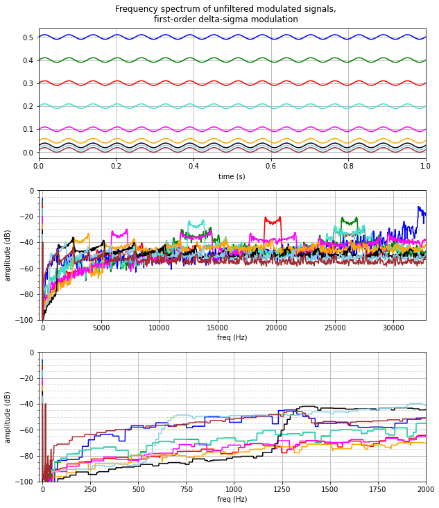
freq_spectrum_sd(dsmod1,[1.0])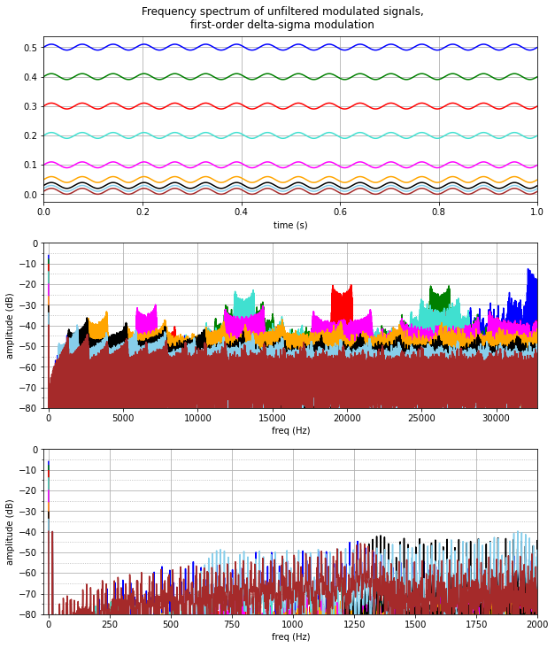
Again, a world of information here in just a simple example. The top plot is the time-series input waveforms. The bottom two plots are the FFT magnitude in decibels, at different frequency scales, and they contain three components:
- the DC component at \( f=0 \)
- the sine-wave component: 0.02 amplitude = -40dB at \( f=16 \) Hz
- modulation noise
The interesting thing here, of course, is the modulation noise. We can’t get rid of it, but the frequency spectrum depends very strongly on the DC offset. In all cases, there’s very little frequency content at 1kHz and below, with the lowest amplitudes nearest to DC. Beyond that, there are different ranges where the quantization noise kicks in, and it depends upon the DC offset. When the DC offset is near 0.5, we get quantization noise near \( f_s/2 \), which makes sense: here the delta-sigma output is chattering back and forth between 0 and 1 on average every other sample. Lower DC offsets have the chattering at lower frequencies since, for example, at a DC offset of 0.2, on average out of every 5 samples, one of them will be a 1 and the rest will be a zero, so we could expect \( f_s/5 \approx 13107 \) Hz in this case. (The same is true for DC offsets greater than 0.5; we haven’t shown them here, but you can use symmetry arguments to show that an input of \( 1-x(t) \) will have identical output to that for \( x(t) \) but with the 0’s and 1’s swapped.)
Note that this is the spectrum of the modulated signals. We haven’t done any filtering, we’re just looking at what a bunch of cleverly-generated pulses is like in the frequency domain.
The frequency spectra (in the middle graph above) have “ears” because the inputs \( x(t) \) are not constant, but are slowly-varying with respect to the delta-sigma output frequency. More specifically, inputs \( x(t) \) are sinusoidal and spend more time at the extremes; we should expect the frequency shape to look similar to a histogram of a sine wave, plotted in log scale:
N = 65536
t = np.arange(N)*1.0/N
a1 = 0.01
w1 = 2*np.pi*16
x = 0.4+a1*np.sin(w1*t)
hcount,hx = np.histogram(x,100)
hx_centers = (hx[:-1]+hx[1:])/2.0
fig,ax = plt.subplots(figsize=(8,6), facecolor='white')
ax.plot(hx_centers,20*np.log10(hcount))
ax.get_yaxis().set_major_locator(ticker.MaxNLocator(12,steps=[1,2,5,10]))
ax.set_ylabel('Relative frequency, dB')
ax.grid(True);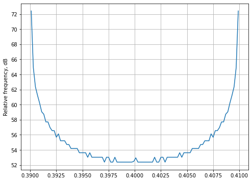
In this case, the “ears” are much larger — about a 20 dB discernible difference between the extremes and the center, whereas in the delta-sigma-modulated spectra, the extremes are about 4-5 dB higher. But it’s the same general effect.
The individual frequency spectra are easier to see if we plot the spectral envelope, that is, the maximum value over some frequency band, so that the plots don’t obscure each other so easily. The envelope_kmax and envelope_min arguments can help; here’s the same spectra but with an envelope over \( 2^6 = 64 \) successive frequency points (envelope_kmax=6) starting at a minimum of 50Hz:
freq_spectrum_sd(dsmod1,[1.0],envelope_kmax=6, envelope_min=50, dBmin=-100)
We can see the spectral distribution of quantization noise fairly easily. In all cases the noise content is lower at low frequencies, and doesn’t really reach -50dB until somewhere between 700-6000Hz depending on the DC offset. We don’t care about the noise content at high frequencies since the intent is to attenuate it with a low-pass filter.
Now, the interesting thing is that when you use a first-order low-pass filter — which is just a plain old RC filter in analog — the error between the filtered output and the filtered input (\( =x^F(t) - y^F(t) \) where I’m using this superscript F to denote a low-pass filter) has a bounded amplitude. The easiest way to think about it, is that at each timestep \( \Delta t \), the filtered output \( y^F(t) \) can take a trajectory upwards with a 1 output, or downwards with a 0 output; the filtered input \( x^F(t) \) is somewhere in between, and the difference between these possible outputs is bounded. We’ll do the math in a second, but here’s what I’m talking about:
a0 = 0.4
di = 0.01
dt_tau = 0.05  # larger than the example above, to show curvature
Ni = 20
ilist = np.arange(0,Ni,di)
fig = plt.figure(figsize=(9,6))
ax = fig.add_subplot(1,1,1)
ax.plot(0,a0,'.')
ai = [a0,a0]
for ii in range(6):
    iifuture = ilist[ilist>=ii]
    iistep = iifuture[iifuture<=ii+1]
    f0 = lambda i,a: a*np.exp(-(i-ii)*dt_tau)
    f1 = lambda i,a: 1-(1-a)*np.exp(-(i-ii)*dt_tau)
    for f,c,w in [(f0,'red',0),(f1,'green',1)]:
        a = ai[1-w]
        ax.plot(iifuture,f(iifuture,a),color=c,linestyle=':')
        ax.plot(iistep,f(iistep,a),color=c)
        ax.plot(ii+1,f(ii+1,a),'.',color=c)
    ai = [f0(ii+1,ai[1]), f1(ii+1,ai[0])]
ax.set_xlim(Ni*-0.01,Ni)
ax.get_xaxis().set_major_locator(ticker.MaxNLocator(12,steps=[1,2,5,10]))
ax.set_xlabel('# steps')
ax.set_ylabel('Filtered output $y^F$')
ax.set_title('Potential trajectories of filtered delta-sigma modulation, first-order low-pass filter');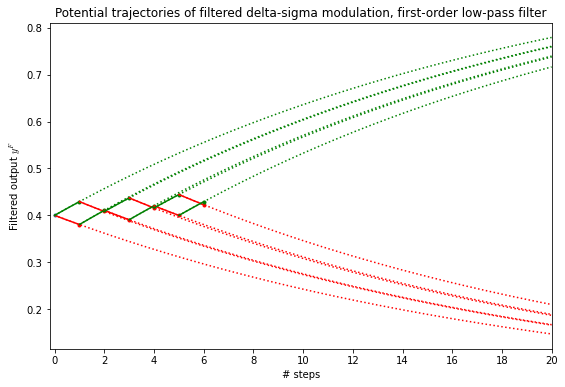
At each step, the possible trajectories form a sort of a herringbone pattern, with 1 outputs forming the upward curves \( y^F = 1-(1-y^F_k)e^{-(t-t_k)/\tau} \) and 0 outputs forming the downward curves \( y^F=y^F_ke^{-(t-t_k)/\tau} \). If we let \( \rho = e^{-\Delta t/\tau} \), then the upwards step change is \( \Delta y^F_+ = 1-\rho(1-y^F_k) \) and the downwards step change is \( \Delta y^F_- = \rho y^F_k \), and the span between them is \( \Delta y^F_+ - \Delta y^F_- = 1-\rho(1-y^F_k) - \rho y^F_k = (1-\rho). \) This is a constant, independent of the filtered output \( y^F \), and it represents the interval in which the filtered input \( x^F \) lies, so the maximum error magnitude is just this interval length \( 1-\rho = 1-e^{-\Delta t/\tau} \approx \Delta t/\tau. \) It turns out that for slowly-changing inputs, the maximum error is about half of this, or \( \approx \Delta t/2\tau. \)
If we look at the first graph I showed in the article, we have \( \Delta t = 0.002 \) and \( \tau=0.05 \), so \( \Delta t/\tau=0.04 \) and half of this is 0.02, which is the error bound amplitude shown in the graph.
Second-order Delta-Sigma Modulation
Things get a little more interesting when we go to second-order delta-sigma modulation. Let’s look at the same kind of error graphs and frequency spectra as in the first-order delta-sigma modulation case.
(We’re going to make one change though: to compare filtered input vs. filtered \( \Delta\Sigma \) modulation, we’ll feed the input into an “unmodulated” version of the modulator, which captures the transfer function \( H(z) \)’s low-pass filtering effect without the quantization.)
Here’s the kernel:
accum1[k] = accum1[k-1] + R*(x[k] - A*y[k-1])
accum2[k] = accum2[k-1] + R*(accum1[k] - B*y[k-1])
y[k] = 1 if accum2[k] >= R*B else 0
We have two accumulators, and two independent feedback gains \( A \) and \( B \).
def dsmod2(x, A, B, ffA=0, ffB=0, ffC=0, R=1, modulate=True):
""" 2nd-order delta-sigma modulation
ffA, ffB, ffC are feedforward terms not normally used
"""
y = np.zeros_like(x)
n = len(y)
accum1 = 0
accum2 = 0
y_out = 0
M = 1 if modulate else 0
for i in range(n):
accum1 += R*(x[i] - A*y_out)
accum2 += R*(accum1 + x[i]*ffA - B*y_out)
q_in = accum2 + x[i]*ffB + accum1*ffC
y_out = (M*(1 if q_in >= R*B else 0)
+(1-M)*q_in)
y[i] = y_out
return y
dsmod2.argformat = ', $B={1:.3f}$'
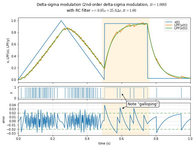
t,x = samplewave()
fig,axes=show_dsmod_samplewave(t,x,dsmod2,args=(1,1.0),
return_handles=True,filter_dsmod=True)
import matplotlib.patches as mpatches
for ax in axes:
yl = ax.get_ylim()
ax.add_patch(mpatches.Rectangle((0.49,yl[0]),0.27,yl[1]-yl[0],
fill=True, color='orange', alpha=0.12,
figure=fig))
axes[2].annotate('',
xy=(0.6, 1.3), xycoords='axes fraction',
xytext=(22, -35), textcoords='offset points',
arrowprops=dict(arrowstyle="-|>",
connectionstyle="arc3",
shrinkA=0,
),
)
axes[2].annotate('Note "galloping"',
fontsize=12,
xy=(0.6, 0.03), xycoords='data',
xytext=(20, 12), textcoords='offset points',
bbox=dict(boxstyle="round", fc="w"),
arrowprops=dict(arrowstyle="-|>",
connectionstyle="arc3",
shrinkA=0,
relpos=(0.1,0.5)),
);
freq_spectrum_sd(dsmod2,(1.0,1.0),envelope_kmax=6, envelope_min=50, dBmin=-100)
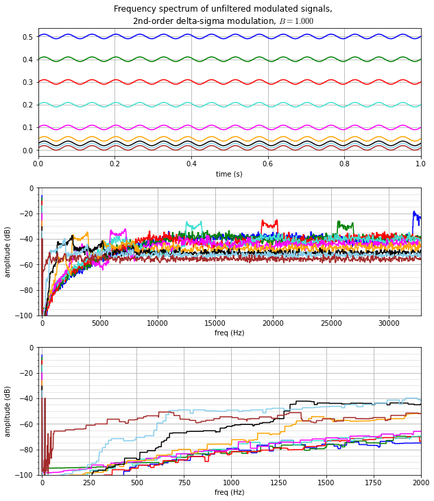
This looks mostly the same as the 1st-order graphs, with a few notable exceptions:
- The noise-shaping at high frequencies (2kHz and higher) is a little better. We can see this in two ways:
- The peak “ears” are 2–5 dB lower with second-order modulation
- Secondary ears are essentially gone in second-order modulation — the remainder of the spectrum is smoother, spreaded more equally as noise.
- Noise-shaping at mid-range frequences (200Hz - 2kHz) is better in most cases, with the exceptions at low DC offset.
- For DC offsets of 0.1 and above, with second-order modulation, the frequency content dropped below a curve leading roughly from -88dB at 500Hz to -66dB at 2kHz.
- With the 1st-order delta-sigma modulation, frequency content of quantization noise at 500Hz and below was in the -80dB to -57dB range; here for the 2nd-order delta-sigma modulator it’s below -88dB except for the very lowest DC offsets (-85dB at \( a_0=0.03 \), -72dB at \( a_0=0.02 \), -57dB at \( a_0=0.0102 \)). The only example that got worse below 500Hz was \( a_0 = 0.02 \), the light blue curve, which increased in the 250Hz – 600Hz range.
- At low frequencies (below 1000Hz) due to DC offsets close to 0 or 1, the error after filtering is worse with 2nd-order delta-sigma modulation than with 1st-order delta-sigma modulation.
- This is visible between 500Hz – 1250Hz at \( a_0=0.03 \) (black curve), 250 – 600Hz at \( a_0 = 0.02 \) (light blue), and below 200Hz at \( a=0=0.0102 \) (brown).
- In part, this is caused by the presence of subharmonic idle tones; note the “galloping” effect in the output and error time-series plots, where the durations between pulses are of alternating lengths (long, short, long, short). We’ll talk about this a little bit later, but one way of thinking about it is that second-order delta-sigma modulation is more “clever” than first-order delta-sigma modulation; the cleverness works well as long as the duty cycle doesn’t get really close to 0 or 1, where the integrators take more time to make changes in the output.
Second-Order Delta-Sigma Modulation Coefficients
One obvious question to ask is where do these A, B coefficients come from, for the 2nd-order delta-sigma modulator. The A coefficient is the same as in the first-order modulator (1 for floating-point values, maximum input for fixed-point values); it determines the low-frequency scaling factor. The B coefficient can be varied as a compromise between stability and quantization noise attenuation, but the A=1, B=1 values seem to be about the best in general, with larger values of B to cover the “galloping” cases where the inputs are close to the limits — again, we’ll talk about this later.
If you’re venturing into 3rd-order or higher delta-sigma modulation, you need to know what you’re doing and get comfortable with z-transforms in order to ensure stability — but 1st-order and 2nd-order delta-sigma are fairly simple to get something workable.
If you really want to get picky, we can analyze the signal and noise transfer functions of a 2nd-order delta-sigma modulator for stability. (If not, just skip ahead past the math.) Remember that \( R=\Delta T/T_0 = 1 \) again, and in this case:
$$Y(z) = H(z)X(z) = R/(1-z^{-1})\left(R/(1-z^{-1})(X(z) - z^{-1}H(z)X(z)) - Bz^{-1}H(z)X(z)\right)$$
$$H(z) = R/(1-z^{-1})\left(R/(1-z^{-1})(1 - z^{-1}H(z)) - Bz^{-1}H(z)\right)$$
$$H(z) + R^2z^{-1}/(1-z^{-1})^2H(z) + BRz^{-1}/(1-z^{-1})H(z) = R^2/(1-z^{-1})^2$$
$$\begin{align}H(z) &= \frac{R^2/(1-z^{-1})^2}{1 + R^2z^{-1}/(1-z^{-1})^2 + BRz^{-1}/(1-z^{-1})} \cr &= \frac{R^2}{(1-z^{-1})^2 + R^2z^{-1} + BRz^{-1}(1-z^{-1})} \cr &= \frac{R^2}{1-2z^{-1}+z^{-2} + R^2z^{-1} + BRz^{-1} - BRz^{-2}} \cr &= \frac{R^2}{1 +(-2+R^2+BR)z^{-1}+(1-BR)z^{-2}} \end{align}$$
$$\begin{align}N(z) &= \frac{1}{1 + R^2z^{-1}/(1-z^{-1})^2 + BRz^{-1}/(1-z^{-1})} \cr &= \frac{(1-z^{-1})^2}{1 +(-2+R^2+BR)z^{-1}+(1-BR)z^{-2}} \end{align}$$
which both have poles at the zeros of \( 1 +(-2+R^2+BR)z^{-1}+(1-BR)z^{-2} \), which occurs when \( z^2 + (-2+R^2+BR)z +(1-BR) = 0 \) or in other words at
$$\begin{align}z &=\frac{2-R^2-BR \pm \sqrt{(2-R^2-BR)^2 - 4(1-BR)}}{2} \cr &=1-(R^2+BR)/2 \pm \sqrt{(1-(R^2+BR)/2)^2 - 1+BR} \cr &=1+R/2\left(-(R+B) \pm \sqrt{(R+B)^2-4}\right). \cr \end{align}$$
This is stable if the poles occur at \( |z| < 1 \).
If \( 0 \le (R+B) < 2 \) then we have a pair of complex poles with \( |z|^2 = (1-R^2/2-BR/2)^2 + R^2/4(4-(R+B)^2) = 1-BR \) which is between 0 and 1 as long as \( B \) and \( R \) are both positive.
If \( (R+B) \ge 2 \) then we have real poles at \( z = 1+R/2(-(R+B) \pm \sqrt{(R+B)^2 - 4}) \). The mess in parentheses is always negative, regardless of the plus/minus sign.
My skills at Grungy Algebra are fading at the moment, so let’s just shown what happens with \( R=1 \). In this case we have \( B>1 \) which produces real poles at \( z = 1-(1+B)/2 \pm \sqrt{(1+B)^2-4}/2 = (1-B)/2 \pm \sqrt{(1+B)^2-4}/2 \). Both poles are within the unit circle as long as \( B<1.5 \); at \( B=1.5 \), the poles are at \( z=-1.0, +0.5 \).
So for the \( R=1 \) case, the system should be stable as long as \( 0 < B < 1.5 \).
At least, that’s the theory, and here are plots of the input and noise transfer functions:
fig = plt.figure(figsize=(9,7))
ax = fig.add_subplot(1,1,1)
f = np.arange(0,0.5,0.001)
# frequency, normalized to 1/delta T
R = 1
for B in [0.5,0.6,0.8,1,1.2]:
    z = np.exp(2j*np.pi*f)
    zinv = 1/z
    denom = 1+(-2+R*R+B*R)*zinv+(1-B*R)*zinv*zinv
    H = R*R/denom
    N = (1-zinv)**2/denom
    line = ax.plot(f,np.abs(H), label='$H(z), B=%.1f$' % B)
    ax.plot(f,np.abs(N),color=line[0].get_color(),linestyle='--',
            label='$N(z), B=%.1f$' % B)
ax.legend(labelspacing=0, fontsize=12, loc='upper left')
ax.set_xlabel('$f\Delta t$', fontsize=16)
ax.set_ylabel('$|H(z)|, |N(z)|$', fontsize=16)
ax.set_ylim(0,4)
ax.set_xlim(0,0.5)
ax.set_title('Input transfer function $H(z)$, noise transfer function $N(z)$',
             fontsize=16);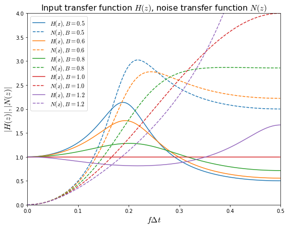
The \( N(z) \) curves at low values of \( f\Delta t \) are almost right on top of each other; they approach the envelope \( \left|N(z)\right| = (\omega\Delta t)^2 = (2\pi f\Delta t)^2 \):
fig = plt.figure(figsize=(9,7))
ax = fig.add_subplot(1,1,1)
f = np.arange(0,0.11,0.0005)
# frequency, normalized to 1/delta T
R = 1
for B in [0.5,0.6,0.8,1,1.25]:
    z = np.exp(2j*np.pi*f)
    zinv = 1/z
    denom = 1+(-2+R*R+B*R)*zinv+(1-B*R)*zinv*zinv
    N = (1-zinv)**2/denom
    ax.plot(f,np.abs(N), label='$N(z), B=%.1f$' % B,linewidth=0.5,
           linestyle='--' if B == 2 else '-')
ax.plot(f,(2*np.pi*f)**2,color='black',linestyle='--',linewidth=1,
       label='limit: $(2\pi f\Delta t)^2$')
ax.legend(labelspacing=0, fontsize=10, loc='upper left')
ax.set_xlabel('$f\Delta t$', fontsize=13)
ax.set_ylabel('$|H(z)|, |N(z)|$', fontsize=13)
ax.set_xlim(0,0.1)
ax.set_ylim(0,0.5);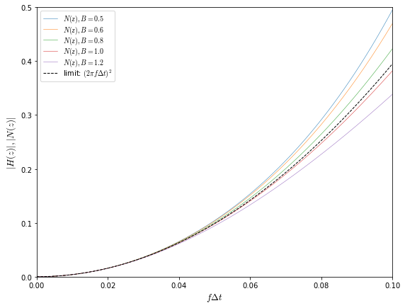
In practice, things are a little different than a linearized model might suggest. Low values of \( B \) can cause large transients.
In the graphs below we look at several values of \( B \), and for calculating the output error we include the transfer function of the linearized (non-modulating) system in the \( LPF(x(t)) \) path to equalize the effects of time delay.
t,x = samplewave()
for B in [0.4, 0.6, 0.8, 1.0, 1.1, 1.2, 1.3, 1.4, 1.49]:
    show_dsmod_samplewave(t,x,dsmod2,args=(1,B),filter_dsmod=True)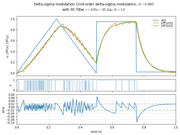
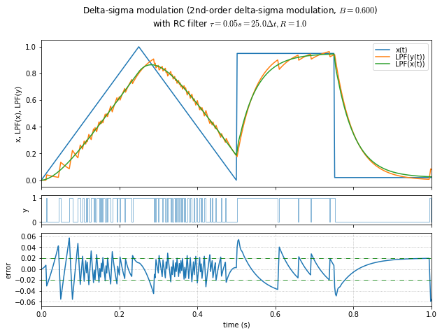
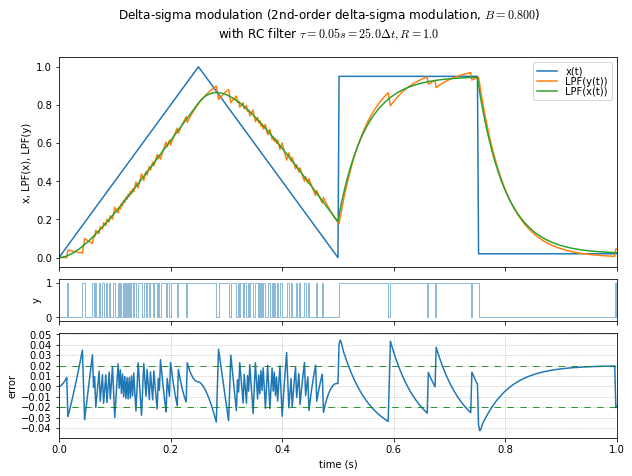
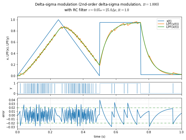
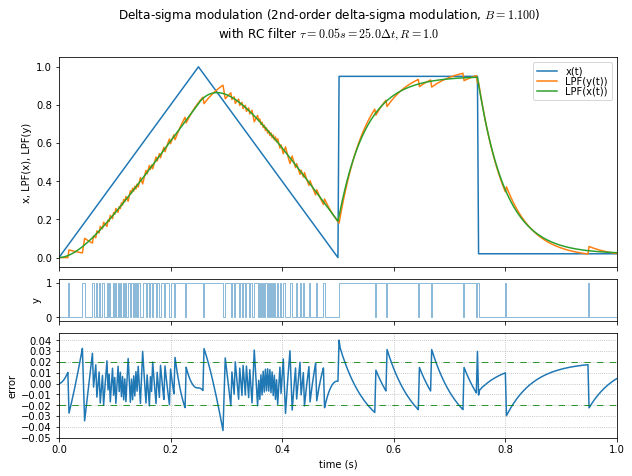

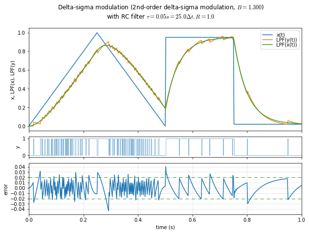
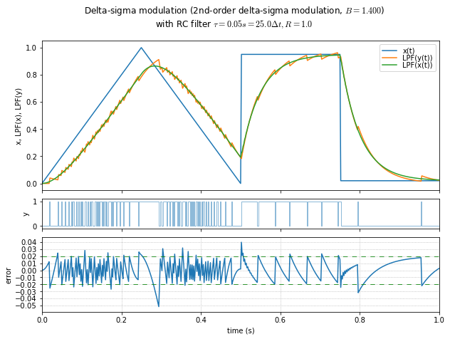
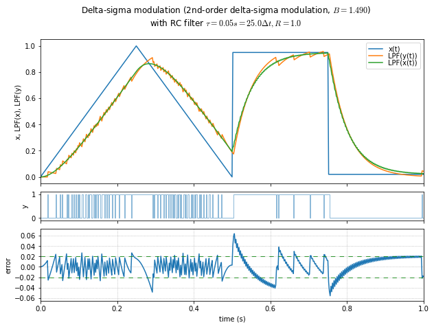
This is an informal demonstration that \( B \) in the 1.2 - 1.4 range seems to be the best at minimizing error and maintaining stability. (Near 1.5, the system is marginally stable and it takes a very long time for oscillations to die out.) If the modulator input is a DC value close to the limits, then lower values of \( B \) allow a “galloping” effect in the output, producing subharmonic idle tones.
Wrapup
OK, so what have we learned today?
-
The “kernel” (defining equation) of a first- and second-order modulator is very simple:
-
first-order:
accum1[k] = accum1[k-1] + R*(x[k] - A*y[k-1]) y[k] = 1 if accum1[k] >= A*R else 0 -
second-order:
accum1[k] = accum1[k-1] + R*(x[k] - A*y[k-1])
accum2[k] = accum2[k-1] + R*(accum1[k] - B*y[k-1])
y[k] = 1 if accum2[k] >= B*R else 0
-
-
The corresponding block diagrams are shown below, and can be linearized by replacing the quantization (comparator) block with an additive source of quantization noise. (In the diagrams, \( R = \Delta t/T_0 \), and I have chosen \( A=1 \); the gain \( A \) is located in the negative input path of the first summing junction.)
- first-order:
- second-order:
-
The value of \( A \) controls the low-frequency gain \( 1/A \) from input to output, and should usually be 1 in floating-point systems.
-
The value of \( R \) controls the integration time constant, but at least for first-order systems, the value of \( R \) affects only the scaling of the integrator, so just use \( R=1 \).
-
The error band of a first-order modulator with timestep \( \Delta t \), when passed through a single-pole RC filter with time constant \( \tau = RC \), is \( \pm\Delta t/2\tau \).
-
Linear analysis assumes that the output quantizer behaves like a source of additive uncorrelated noise, in which we can determine the input-output transfer function \( H(z) \) and the quantization noise transfer function \( N(z) \).
-
We can look at the frequency spectrum of modulated signals, and as long as the inputs aren’t too close to 0 or \( A \), then the noise gets suppressed at lower frequencies and pushed out to higher frequencies; the noise transfer function \( N(z) \) behaves roughly as \( \left|N(\omega)\right| \approx \omega \Delta t \) for first-order modulation and \( \left|N(\omega)\right| \approx (\omega \Delta t)^2 \) for second-order modulation.
-
For second-order systems, \( B \) should be chosen in the 1.0 - 1.4 range, with higher values used to reduce a “galloping” behavior.
Next time we’ll look at some of the tradeoffs of output filters for delta-sigma modulation.
© 2019, 2023 Jason M. Sachs, all rights reserved.