PID Without a PhD

I both consult and teach in the area of digital control. Through both of these efforts, I have found that while there certainly are control problems that require all the expertise I can bring to bear, there are a great number of control problems that can be solved with the most basic knowledge of simple controllers, without resort to any formal control theory at all.

This article will tell you how to implement a simple controller in software and how to tune it without getting into heavy mathematics and without requiring you to learn any control theory. The technique used to tune the controller is a tried and true method that can be applied to almost any control problem with success.

Author's Note

This article teaches you how to implement control systems without resort to much mathematics. While the techniques shown here will work in a great many cases, in a great many cases they will not. In those cases I recommend that you study control theory starting with my book, Applied Control Theory for Embedded Systems by Tim Wescott, or that you find a qualified consultant. 

If you find this paper informative but would like to see the discussion with the math in, the book is for you.

If you find this paper informative but you feel that you need to have a control systems expert to help you with your project, I may be available. My contact information is on my website, and I'll be happy to talk to you.

Overview

This paper will describe the PID controller. This type of controller is extremely useful and, along with some related controllers described here, is possibly the most often used controller in the world. PID control has been in use since the 19th century in various forms [Max68]. It has enjoyed popularity as a purely mechanical device, as a pneumatic device, and as an electronic device. The digital PID controller using a microprocessor has recently come into its own in industry. As you will see, it is a straightforward task to embed a PID controller into your code.

Control Loops

Before we go into the anatomy of a PID controller, let us look at the anatomy of the control loop in which it lives. The drawing in figure 1 shows a block diagram of a control loop. Some command is given to a controller, and the controller determines a drive signal to be applied to the plant (A “plant” is simply a control system engineer's name for the thing that we wish to control. I believe that it comes from “steam plant”, however I do not know for sure). In response to being driven, the plant responds with some behavior. In a closed-loop control system such as a PID loop, the plant behavior is measured, and this measurement is fed back to the controller, which uses it along with the command to determine the plant drive.

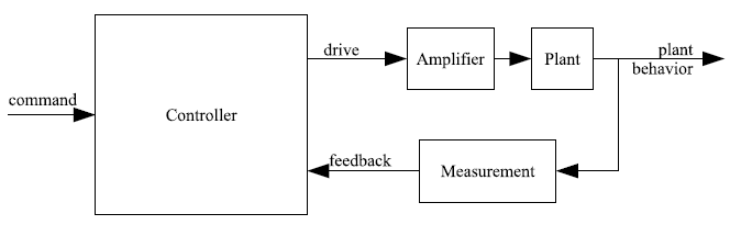
Figure 1: Anatomy of a control loop. 

PID Control

The "PID" in "PID Control" stands for "Proportional, Integral, Derivative". These three terms describe the basic elements of a PID controller. Each of these elements performs a different task and has a different effect on the functioning of a system.

In a typical PID controller these elements are driven by a combination of the system command and the feedback signal from the thing that is being controlled (usually referred to as the "Plant"). Their outputs are added together to form the system output.

The block diagram in figure 2 shows the structure of a basic PID controller that we will use throughout the text. The plant feedback is subtracted from the command signal to generate an error. This error signal drives the proportional and integral elements. The derivative element is driven only from plant feedback. The resulting signals are added together and used to drive the plant. I haven't described what these elements do yet---we'll get to that later. I've included an alternate placement for the proportional element (dotted lines). This can be a better place for the proportional element, depending on how you want the system to respond to commands.

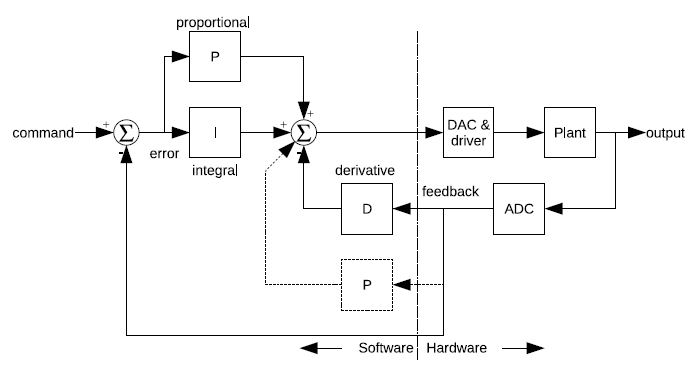
Figure 2: Block diagram of PID controller.

Example Plants

To ground this discussion in reality I'll use some example systems. I'll use three example plants throughout this article. These are the sort of plants that have been brought to me by students or customers again and again. I'll use these systems to show the effects of the various controllers on different plants. 

In spite of promising to leave out the math, I've included differential equations that describe the behavior of these systems. If you're comfortable with the math it will help you to understand the problem. If you aren't, skip them.

I'll use three example plants: A motor driving a gear train, a precision positioning system, and a thermal system. Each has different characteristics and each requires a different control strategy to get the best performance.

Motor & Gear

The first example plant is a motor driving a gear train, with the output position of the gear train being monitored by a potentiometer or some other position reading device. You might see this kind of mechanism driving a carriage on a printer, or a throttle mechanism in a cruise control system or almost any other moderately precise position controller. Figure 3 shows a diagram of such a system. The motor is driven by a voltage which is commanded by software and applied to its terminals. The motor output is geared down to drive the actual mechanism. The position of this final drive is measured by the potentiometer (“pot” in the figure) which outputs a voltage proportional to the motor position.

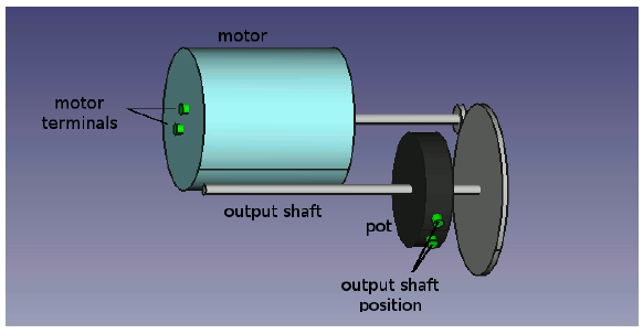
Figure 3: Motor & Gear

In the absence of external influences, a DC motor driven by a voltage will go at a constant speed, proportional to the applied voltage. Usually the motor armature has some resistance that limits its ability to accelerate, so the motor will have some delay between the input voltage changing and the speed changing. The gear train takes the movement of the motor and multiplies it by a constant. Finally, the potentiometer measures the position of the output shaft. 

The response of the motor position to the input voltage can be described by the equation

$$ \frac{d^{2}}{dt^{2}}\theta_{m}=-\frac{1}{\tau_{0}}\left(\frac{d}{dt}\theta_{m}+k_{v}V_{m}\right) \tag{1}$$

where the time constant $ \tau_{0} $ describes how quickly the motor settles out to a constant speed when its supply voltage changes. The $ k_{v} $ term is the motor gain; it tells how fast the motor will turn in response to a given voltage. The term $ \tau_{0} $ has units of seconds; the $ k_{v} $ term here has units of degree/second/volt but usually shows up on motor data sheets in RPM/volt. 

Once you know the motor behavior, you can look at the effect of the gear train and potentiometer. Mathematically, the effect of the gear train is to multiply the motor angle by a constant; it is represented below by $ k_{g} $. Similarly, the potentiometer acts to multiply the gear angle by a constant, $ k_{p} $, which scales the output angle and changes it from an angle to a voltage (thus $ k_{p} $ has units of volts/degree).

A useful concept when working with control systems is the “step response”. A system's step response is just the behavior of the system output in response to an input that goes from zero to some constant value at time $ t=0 $. We're dealing with fairly generic examples here so I'll normalize the step input as a fraction of full scale, with the step going from 0 to 1 (this normalized input step makes the response the “unit step response”). Figure 4 shows the step response of the motor and gear combination. I'm using a time constant value $ \tau_{0}=0.2 seconds $. This figure shows the step input and the motor response. The response of the motor starts out slowly due to the time constant, but once that is out of the way the motor position ramps at a constant velocity.

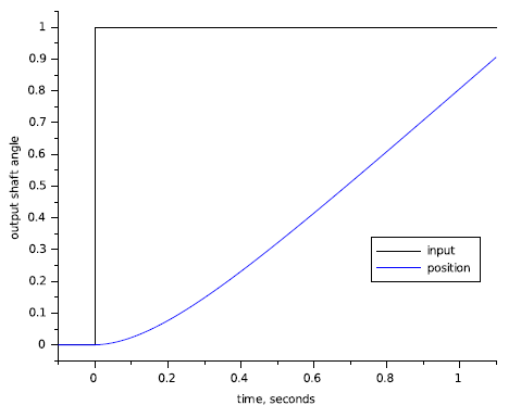
Figure 4: Motor step response.

Precision Actuator

It is sometimes necessary to control the position of something very precisely. A precise positioning system can be built using a freely moving mechanical stage, a speaker coil (a coil and magnet arrangement) and a non-contact position transducer.

I have worked with this sort of mechanism to stabilize an element of an optical system, however, such systems show up in the areas of semiconductor processing, high-end printers, and various other industries. The drawing in figure 5 shows an example of such a system. Software commands the current in the coil. This current sets up a magnetic field which exerts a force on the magnet. The magnet is attached to the stage, which moves with an acceleration proportional to the coil current. Finally, the stage position is monitored by a non-contact position transducer.

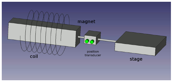
Figure 5: Speaker Coil Assembly.

With this arrangement the force on the magnet is independent of the stage motion. Fortunately this isolates the stage from external effects. Unfortunately the resulting system is very "slippery", and can be a challenge to control. In addition, the electrical requirements to build a good current-output amplifier and non-contact transducer interface can be challenging. You can expect that if you are doing a project like this you are a member of a fairly talented team (or that you're heading toward a very educational disaster).

The equations of motion for this system are fairly simple. The force on the stage is proportional to the drive command and nothing else, so the acceleration of the system is exactly proportional to the drive.

$$ \frac{d^{2}}{dt^{2}}x=\frac{k_{i}}{m}i_{c},\;V_{p}=k_{t}x \tag{2}$$

where $ V_{p} $ is the transducer output, $ k_{i} $ is the coil force constant in newtons/amp (or pounds/amp), $ k_{t} $ is the transducer gain in volts/meter (or volts/foot), and $ m $ is the total mass of the stage, magnet and the moving portion of the position transducer in appropriate units.

The step response of this system by itself is a parabola, as shown in figure 6. As we will see later this makes the control problem more challenging because of the sluggishness with which the stage starts moving, and its enthusiasm to keep moving once it gets going.

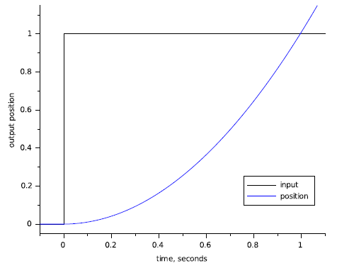
Figure 6: Speaker-coil actuator step response.

Temperature Control

The third example plant I'll use is a heater. A diagram of an example system is shown in figure 7. The vessel is heated by an electric heater, and the temperature of its contents is sensed by a temperature sensing device.

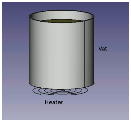
Figure 7: A heating system.

This example system is highly oversimplified. Thermal systems tend to have very complex responses, which can be difficult to characterize well. I'm going to ignore quite a bit of detail and give a very approximate model. The equations I'm using are here. This model will be accurate enough for our purposes, and does not require advanced training in control systems to understand.

$$ \begin{aligned}\frac{d^{2}}{dt^{2}}T_{h}=-\left(\frac{1}{\tau_{1}}+\frac{1}{\tau_{2}}\right)\frac{d}{dt}T_{h}-\frac{T_{h}}{\tau_{1}\tau_{2}}+\frac{k_{h}V_{d}+T_{a}}{\tau_{1}\tau_{2}}\end{aligned} \tag{3}$$

where $ V_{d} $ is the input drive, $ T_{h} $ is the temperature $ \tau_{1} $ and $ \tau_{2} $ are time constants with units of seconds (arbitrarily chosen for the purpose of illustration), $ k_{h} $, the heater constant, has units of degrees C per volt, $ T_{h} $ is the measured temperature and $ T_{a} $ is the ambient temperature.

The plot in figure 8 shows the step response of the system to both to a change in $ V_{d} $ and to a change in ambient temperature. I've used time constants of $ \tau_{1}~=~0.1s $ and $ \tau_{2}~=~0.3{s} $. The response tends to settle out to a constant temperature for a given drive but it can take a great deal of time doing it. In addition, this example, unlike the motor example and the speaker-coil example, takes a disturbance input into account. Here, the disturbance is the ambient temperature, which the system will respond to the same as it responds to changes in the drive level.

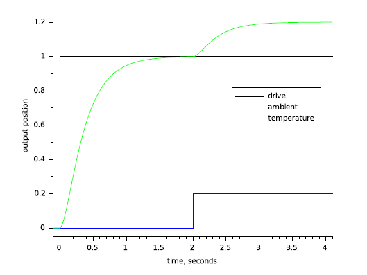
Figure 8: Heater response to drive and ambient temperature.

Controllers

Now that we have some example plants to play with, we can try controlling these plants with various variations of proportional, integral, and derivative control. In this section, I will show you how to write various different controllers, and how these controllers will affect the behavior of the system in closed loop.

The elements of a PID controller such as the one below can take their input either from the measured plant output or from the error signal (which is the difference between the plant output and the system command). In the controller that I develop below I will use both of these sources. 

All the example controller code uses floating point arithmetic to keep implementation details out of the discussion. For an actual system, however, it is quite possible that you would want to use some sort of fixed-point arithmetic to limit your required processor speed [Wes06]. If you do end up using floating point for this task, you will almost certainly need to use double-precision floating point---take this into consideration when you calculate the amount of processor loading your algorithm will introduce.

I'm going to assume a controller function call as shown below. The function UpdatePID takes the error and the actual plant output as inputs, it modifies the PID states (in pid), and it returns a drive value to be applied to the plant. As the discussion evolves, you'll see how the data structure and internals of the function shape up.

typedef double real_t;  // this almost certainly needs to be double
real_t UpdatePID(SPid * pid, real_t error, real_t position)
{
.
.
.
}

The reason I pass the error to the PID update routine instead passing the command is that sometimes you want to play tricks with the error. Leaving the error calculation out in the main code makes the application of the PID more universal. This function will get used like this:

.
.
position = ReadPlantADC();
drive = UpdatePID(&plantPID, plantCommand - position, position);
DrivePlantDAC(drive);
.
.

Proportional

Proportional control is the easiest feedback control to implement, and simple proportional control is probably the most common kind of control loop. A proportional controller is just the error signal multiplied by a constant and fed out to the drive. The proportional term gets calculated with the following code within the function UpdatePID:

real_t pTerm;
.
.
.
pTerm = pid->propGain * error;
.
.
.
return pTerm;

Figure 9 shows what happens when you add proportional feedback to the motor and gear system. For small gains (propGain or $ k_{p}=1 $) the motor goes to the correct target, but it does so quite slowly. Increasing the gain ($ k_{p}=2 $) speeds up the response to a point. Beyond that point ($ k_{p}=5 $, $ k_{p}=10 $) the motor starts out faster but overshoots the target. In the end the system doesn't settle out any quicker than it would have with lower gain, but there is more overshoot. If we were to keep increasing the gain we would eventually reach a point where the system just oscillated around the target and never settled out: the system would be unstable.

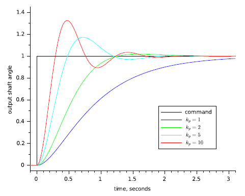
Figure 9: Motor with proportional control.

The reason the motor and gear start to overshoot with high gains it because of the delay in the motor response. If you look back at Figure 4, you can see that the motor position doesn't start ramping up immediately. This delay, plus high feedback gain, is what causes the overshoot seen in Figure 9.

Figure 10 shows the response of the precision actuator with proportional feedback only. Here the situation is worse: proportional control alone obviously doesn't help this system. There is so much delay in the plant that no matter how low the gain is the system will oscillate. As the gain is increased the frequency of the output will increase, but the system just won't settle. Proportional-only control is inadequate for this plant.

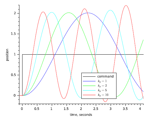
Figure 10: Precision actuator with proportional control.

Figure 11 shows what happens when you use pure proportional feedback with the temperature controller. I'm showing the system response with a disturbance due to a change in ambient temperature at $ t=2 $ seconds. Even without the disturbance you can see that proportional control doesn't get the temperature to the desired setting; with the disturbance you can see that the loop is susceptible to external effects. Increasing the gain helps with both the settling to target and with the disturbance rejection, but even with $ k_{p}=10 $ the output is still below target, and you are starting to see a strong overshoot that continues to travel back and forth for some time before settling out (this is called "ringing").

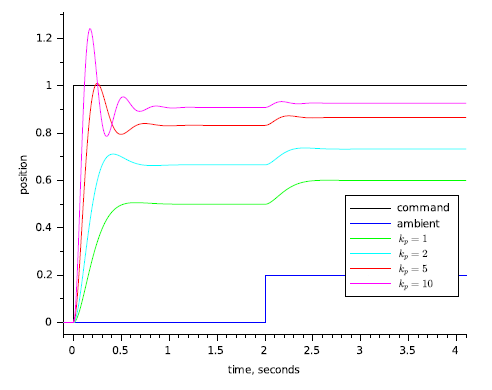
Figure 11: Heater with proportional control.

As the examples above show, a proportional controller alone can be useful for some plants, but for others it may not help, or it may not help enough. Plants that have too much delay, like the precision actuator, can't be stabilized with proportional control. Some plants, like the temperature controller, cannot be brought to the desired set point. Plants like the motor and gear combination may work, but they may need to be driven faster than is possible with proportional control alone, and they may be subject to external disturbances that proportional control alone cannot compensate for. To solve these control problems you need to add integral or differential control or both.

Integral

Integral control is used to add long-term precision to a control loop. It is almost always used in conjunction with proportional control. 

The code to implement an integrator is shown below. The integrator state (integratState) is the sum of all the preceding inputs. The parameters integratMin and integratMax are the minimum and maximum allowable integrator state values.

real_t iTerm;
.
.
.
// calculate the integral state with appropriate limiting
pid->integratState += error;
// Limit the integrator
if (pid->integratState > pid->integratMax) 
{
  pid->integratState = pid->integratMax;
}
else if (pid->integratState < pid->integratMin) 
{
  pid->integratState = pid->integratMin;
}
// calculate the integral term
iTerm = pid->integratGain * pid->integratState;
.
.
.

Integral control by itself usually decreases stability, or destroys it altogether. Figure 12 shows the motor and gear with pure integral control (propGain = 0) and a variety of integrator gains (integratGain or $ k_{i} $). This system simply doesn't settle, no matter how low you set the integral gain. Like the precision actuator with proportional control, the motor and gear system with integral control along will oscillate with bigger and bigger swings until something hits a limit (hopefully the limit isn't breakable).

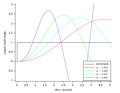
Figure 12: Motor with pure integral control.

I'm not even showing the effect of using integrator control on the precision actuator system. Why? Because the precision actuator system can't even be stabilized with a proportional controller. There is simply no integral gain that could be chosen that would make the system stable. We'll pick up on the precision actuator system later on, when we talk about derivative control.

Figure 13 shows the temperature control system with pure integral control. This system takes a lot longer to settle out than the same plant with proportional control (see Figure 11), but notice that when it does settle out it settles out to the target value ‑ even the undesired response from the disturbance goes to zero eventually. Chances are this is too slow for you, but if your problem at hand didn't require fast settling, even this simple of a controller might be workable.

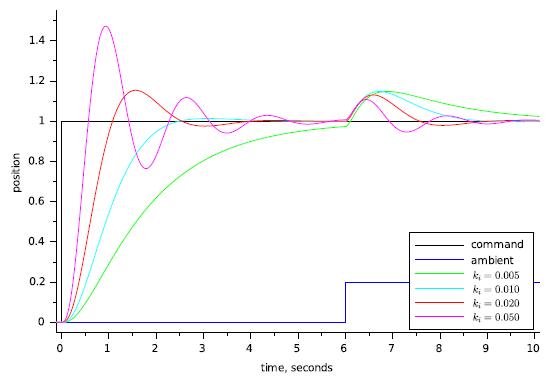
Figure 13: Heater with integral-only control.

Figure 13 shows why we use an integral term. The integrator state "remembers" all that has gone on before, which is what allows the controller to cancel out any long term errors in the output. This same memory also contributes to instability ‑ the controller is always responding too late, after the plant has gotten up speed. What the two systems above need to stabilize them is a little bit of their present value, which you get from a proportional term.

Proportional-Integral Control

We've seen that proportional control by itself has limited utility, and that while integral control by itself can vastly improve the steady-state behavior of a system, it often destroys stability. It would be nice, then, if there was a way to combine the steady-state improvements of integral control with the improvements of proportional control. Fortunately, there is. It is called proportional-integral control.

Figure 14 shows the motor and gear with the proportional and integral (PI) control. Compare this with figure 9 and figure 12. The position takes longer to settle out than the system with pure proportional control, but unlike the motor with pure integral control it does settle out, and the system will not settle to the wrong spot.

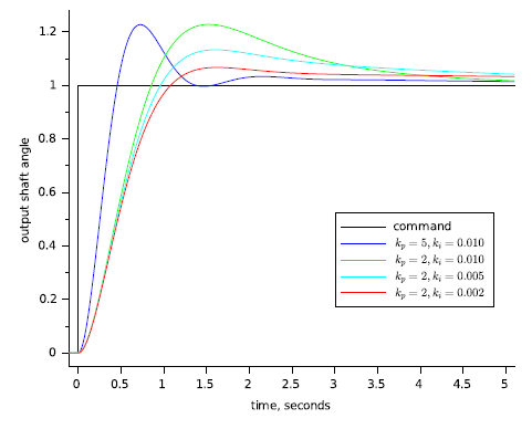
Figure 14: Motor with proportional-integral control.

For many systems this is exactly the right behavior: often it is far more important for a system to settle out to exactly the correct position than for it to settle quickly to the wrong position. Questions of which is better depend on the problem at hand, and selecting the correct design criteria is important for success.

Figure 15 shows what happens when you use PI control on the heater system. The heater still settles out to the exact target temperature as with pure integral control (Figure 13), but with PI control it settles out 2 to 3 times faster. This figure shows operation pretty close to the limit of the speed that you can attain with PI control of this plant.

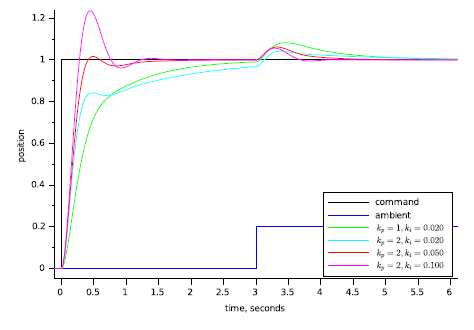
Figure 15: Heater with proportional-integral control.

Before we leave the discussion of integrators, there are two more things I need to point out. First, since you are adding up the error over time, the sampling time that you are running becomes important. Second, you need to pay attention to the range of your integrator to avoid windup.

The rate that the integrator state changes is equal to the average error times the integrator gain times the sampling rate. Because the integrator tends to smooth things out over the long term you can get away with a somewhat uneven sampling rate, but it needs to average out to a constant value. At worst, your sampling rate should vary by no more than $ \pm20\% $ over any ten sample interval. You can even get away with missing a few samples as long as your average sample rate stays within bounds. None the less, for a PI controller I prefer to have a system where each sample falls within $ \pm1\% $ to $ \pm5 $ of the correct sample time, and a long-term average rate that is right on the button.

If you have a controller that needs to push the plant hard your controller output will spend significant amounts of time outside the bounds of what your drive can actually accept. This condition is called saturation. If you use a PI controller, then all the time spent in saturation can cause the integrator state to grow (wind up) to very large values. When the plant reaches the target, the integrator value is still very large, so the plant drives beyond the target while the integrator unwinds and the process reverses. This situation can get so bad that the system never settles out, but just slowly oscillates around the target position.

Figure 16 illustrates the effect of integrator windup. I used the motor/controller of Figure 13, and limited the motor drive to $ \pm0.2 $. Not only is controller output much greater than the drive available to the motor, but the motor shows severe overshoot. The motor actually reaches its target at around 5 seconds, but it doesn't reverse direction until 8 seconds, and doesn't settle out until 15 seconds have gone by.

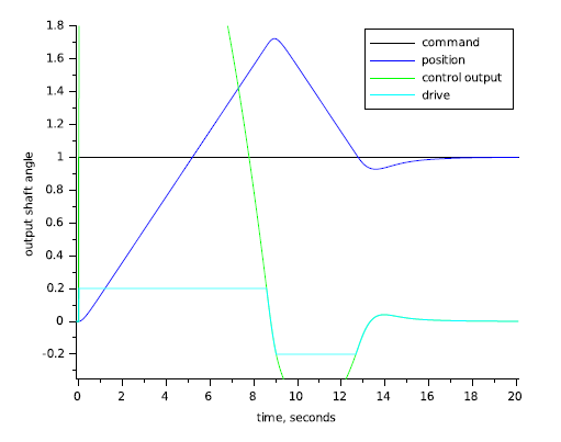
Figure 16: Motor with PI control and windup.

There are many good ways to deal with integrator windup (windup, and anti-windup methods, are treated in more depth in [Wes06]). Perhaps the easiest and most direct way to deal with integrator windup is to limit the magnitude of the integrator state to as I showed in my code example above. Figure 17 shows what happens when you take the system in Figure 16 and limit the integrator term to the available drive output. The controller output is still large (because of the proportional term), but the integrator doesn't wind up very far and the system starts settling out at 5 seconds, and finishes at around 6. Note that with the code example above you must scale integratMin and integratMax whenever you change the integrator gain. Usually you can just set the integrator minimum and maximum so the integrator output matches the drive minimum and maximum. If you know your disturbances will be small and you want quicker settling you can limit the integrator further.

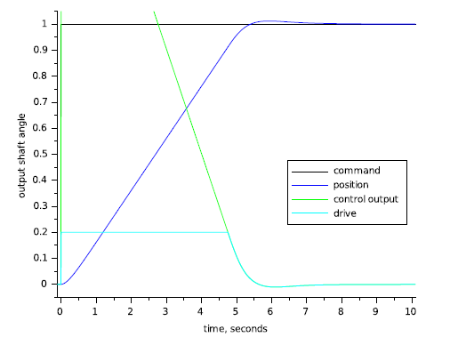
Figure 17: Motor with output limiting and anti-windup.

Derivative

I didn't even show the precision actuator in the previous section. This is because the precision actuator cannot be stabilized with PI control. In general if you cannot stabilize a plant with proportional control you cannot stabilize it with PI control.

We know that proportional control deals with the present behavior of the plant, and that integral control deals with the past behavior of the plant. If we had some element that predicts the plant behavior then this might be used to stabilize the plant. A differentiator does this.

The listing below shows how to code the derivative term of a PID controller. I prefer to use the actual plant position rather than the error because this makes for smother transitions when the command value changes. The derivative term itself is just the last value of the position minus the current value of the position. This gives you a rough estimate of the velocity (delta position / sample time), which predicts where the position will be in a while.

real_t dTerm;
.
.
.
dTerm = input - pid->derState;
pid->derState = input;
.
.
.

With differential control you can stabilize the precision actuator system. Figure 18 shows the response of the precision actuator system with proportional and derivative (PD) control for various values of proportional gain and derivative gain (derGain, $ k_{d} $). This system settles in less than 1/2 or a second, compared to multiple seconds for the other systems.

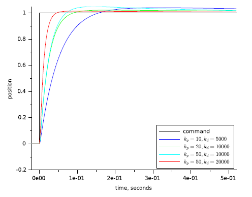
Figure 18: Precision Actuator with PD control.

Figure 19 shows the heating system with PID control. You can see the performance improvement to be had by using full PID control with this plant.

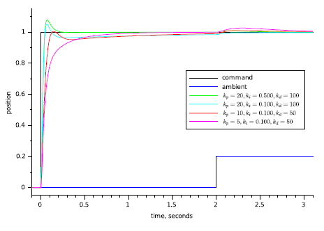
Figure 19: Heater with PID control.

Differential control is very powerful, but it is also the most problematic of the control types presented here. The three problems that you will most likely experience are sampling irregularities, noise, and high frequency oscillations.

When I presented the code for a differential element I mentioned that the output is proportional to the position change divided by the sample time. If the position is changing at a constant rate but your sample time varies from sample to sample then you will get noise on your differential term. Since the differential gain is usually high, this noise will be amplified a great deal.

Noise can be a big problem when you use differential control, to the extent that it often bars you from using differential control without making modifications to your system's electrical or mechanical arrangement to deal with it at the source. A full treatment of noise and its effects is beyond the scope of this paper.

For example, noise is usually spread pretty evenly across the frequency spectrum. Control commands and plant outputs, however, usually have most of their content at lower frequencies. Proportional control passes noise through unmolested. Integral control averages its input signal, which tends to kill noise. Differential control enhances high frequency signals, so it enhances noise. Look at the differential gains that I've set on the plants above, and think of what will happen if you have noise that makes each sample a little bit different. If you multiply that little bit by a differential gain of 2000 you could very well have serious problems.

When you use differential control you need to pay close attention to even sampling. At worst you want the sampling interval to be consistent to within 1% of the total at all times, the closer the better. If you can't set the hardware up to enforce the sampling interval then design your software to sample with very high priority. You don't have to actually execute the controller with such rigid precision ‑ just make sure that the actual ADC conversion happens at the right time. If necessary put all of your sampling in an ISR or very high-priority task, then execute the control code in a more relaxed manner.

You can low-pass filter your differential output to reduce the noise, but if done incorrectly this can severely affect its usefulness. The theory on how to do this and how to determine if it will work is well beyond the scope of this article, although I do address it in [Wes06]. Probably the best that you can do about this problem is to look at how likely you are to see any noise, how much it will cost to get quiet inputs, and how badly you need the high performance that you get from differential control. Once you know these things you can avoid differential control altogether, talk your hardware folks into getting you a lower noise input, or look for a control systems expert.

The Complete Controller

Here is the full text of the PID controller code.

typedef struct
{
  real_t derState;      // Last position input
  real_t integratState; // Integrator state
  real_t integratMax,   // Maximum and minimum
         integratMin;   // allowable integrator state
  real_t integratGain,  // integral gain
         propGain,      // proportional gain
         derGain;       // derivative gain
} SPid;
real_t UpdatePID(SPid * pid, real_t error, real_t position)
{
  real_t pTerm, dTerm, iTerm;
  pTerm = pid->propGain * error; // calculate the proportional term
  // calculate the integral state with appropriate limiting
  pid->integratState += error;
  // Limit the integrator state if necessary
  if (pid->integratState > pid->integratMax)
  {
    pid->integratState = pid->integratMax;
  }
  else if (pid->integratState < pid->integratMin)
  {
    pid->integratState = pid->integratMin;
  }
  // calculate the integral term
  iTerm = pid->integratGain * integratState;
  // calculate the derivative
  dTerm = pid->derGain * (pid->derState - position);
  pid->derState = position;
  return pTerm + dTerm + iTerm;
}

Tuning

Tuning the PID Controller

The very nice thing about tuning a PID controller is that you don't need to have a good understanding of formal control theory to do a fairly good job of it. Ninety percent of the closed-loop controller applications in the world do very well indeed with a controller that is only tuned fairly well, so you're in luck. I have received a number of emails from people who have used the techniques described here and who were quite satisfied with their results. These techniques don't always work, of course: in some cases you need to gain a deeper understanding of control system theory, such as you would get from my book or from attending one of my longer seminars.

If you can, hook your system up to some test equipment, or write in some debug code to allow you to look at the appropriate variables. If your system is slow enough you can just spit the appropriate variables out on a serial port and graph them with a spreadsheet. If you are tuning something motorized you may be able to just watch it's behavior. Ideally, you want to be able to look at the drive output and the plant output, to get graphs similar to the ones earlier in this paper. In addition, you also want to apply a changing command---preferably a square-wave---to your system. It is fairly easy to write some test code that will generate a suitable test command.

Once you get the setup ready, set all gains to zero. If you suspect that you will not need differential control (like the motor and gear example or the thermal system) then skip down to the section that discusses tuning the proportional gain. Otherwise start by adjusting your differential gain.

Adjusting Derivative Gain

The way the controller is coded you cannot use derivative control alone. If you can, set your proportional gain to a value that's low enough to prevent oscillation, or at least so that the system is oscillating much more slowly than you want it to react when it is tuned. 

Check to see how the system works. If it oscillates with proportional gain you should be able to cure it with differential gain. If it doesn't oscillate, but it appears that the proportional control term is working, consider yourself lucky.

Now put in some derivative gain. Start with about 100 times more derivative gain than proportional gain. Watch your drive signal while you stimulate the system. If the system oscillates under derivative control when it did not oscillate under proportional control alone, or if the system oscillates much faster when you dial in some derivative gain, back the derivative gain off by factors of two until it stops.

If you did not need to decrease the derivative gain to make the system stop oscillating, start increasing it gain until you do see oscillation, excessive noise or excessive (more than 50%) overshoot on the drive or plant output. Note that the oscillation from too much derivative gain is much faster than the oscillation from not enough, or from too much proportional gain. I like to push the gain up until the system is on the verge of oscillation, then back the gain off by a factor of 2 or 4. Make sure the drive signal still looks good. At this point your system will probably be settling out very sluggishly, so its time to tune the proportional and integral gains.

Adjusting Proportional Gain

If you have nonzero derivative gain in your system, a good starting value for the proportional gain is $ \frac{1}{100} $ of the derivative gain value. This may cause the system to oscillate, it may leave the system very sluggish, but it should be a starting point.

If you are not using derivative action in the system, find a starting value for the proportional gain. In most control systems, a gain of between 1 and 100 is a good point to start. With this initial value your system will probably either show terribly slow performance or it will oscillate. 

Now that you have an initial guess for the proportional gain, see if you have oscillation. If you see oscillation drop the proportional gain by factors of 8 or 10 until the oscillation stops. If you don't see oscillation, increase the proportional gain by factors of 8 or 10 until you start seeing oscillation or excessive overshoot. Once you are close, fine tune the proportional gain by factors of two until you see oscillation, then back the gain off by a factor of two or four.

Adjusting Integrator Gain

Once you have your proportional gain set, start adjusting integral gain. 

If you are using derivative gain, a good starting value for the integrator gain is to set it smaller than the proportional gain by the same ratio as proportional gain to derivative gain. For example, if you have a derivative gain of 1000 and a proportional gain of 10 (a 100:1 ratio), set the starting integrator gain to 0.1.

If you are not using derivative gain, a good starting value for the integrator gain will be around $ \frac{1}{100} $ of the proportional gain. Try this gain. If you see oscillation, decrease the integrator gain by steps of 8 or 10 until the oscillation goes away. If you don't see oscillation, increase the integrator gain by steps of 8 or ten until you do. From this point, try to find the gain where the system just breaks into oscillation, and then back the gain off by a factor of 2 or 4.

The hardest part

When you have gone through this sequence exactly once: find the derivative gain, find the proportional gain, and then find the integrator gain, you must stop. Do not go back and tweak the gains. Doing so is a very good way to fool yourself into thinking that you've improved performance, while actually shoving the system into a corner of it's operating envelope that may well render it a “lab queen” that will only work under the best of circumstances.

If you go through this adjustment procedure, and you stop, and you find that the performance of your control loop is not sufficient to meet product requirements, then you need to either use more advanced control loop design techniques (see [Wes06]), you need to increase the underlying performance of the parts of your control loop, you need to hire a control system expert to help you out, or some combination of the above.

Other Issues

Doing Math

I mentioned it in passing above, but you do not have to do your computations in floating point. In fact, even at this writing (spring of 2016), you must pay a premium for processors that can do fast double-precision floating point. Most embedded processors can do integer arithmetic much faster than they can do floating point, and the tradeoff between the development time to use fixed-point math, and the savings in processor loading, is often a good one.

Unless you are working on a project with very critical performance parameters you can often get by with control gains that are within a factor of two of the "correct" value. This means that---if you are doing your computations with integer math---you can do all your "multiplies" with shifts. With smaller processors that do not do multiplication in hardware, this can lead to a dramatic decrease in the processor time taken for each iteration of the control loop. This, in turn, will lead to a matching increase in performance, or a decrease in processor performance requirements.

Determining Sampling Rates

So far I've only talked about sample rates in terms of how consistent they need to be, but I haven't told you how to decide ahead of time what the sample rate needs to be. If your sampling rate is too low you may not be able to achieve the performance you want, because of the added delay of the sampling. If your sampling rate is too high you will create problems with noise in your differentiator and overflow in your integrator.

The rule of thumb for digital control systems is that the sample time should be between 1/10th and 1/100th of the desired system settling time. System settling time is the amount of time from the moment that the drive comes out of saturation until the control system has effectively settled out. If you look at Figure 16, the controller comes out of saturation at about 5.2 seconds, and has settled out at around 6.2 seconds. If you can live with the one second settling time you could get away with a sampling rate as low as 10Hz.

You should treat the sampling rate as a flexible quantity. Anything that might make the control problem more difficult would indicate that you should raise the sampling rate. Factors such as having a difficult plant to control, or needing differential control, or needing very precise control would all indicate raising the sampling rate. If you have a very easy control problem you could get away with lowering the sampling rate somewhat (I would hesitate to lower it below 5 times the frequency of interest). If you aren't using a differentiator and you are careful about using enough bits in your integrator you can get away with sampling rates 1000 times faster than you intended settling time.

Formal Math

An issue that I haven't taken up is how to use formal control theory. to solve this sort of control system design problem. The reason for this is twofold: one is because I promised not to in the abstract; the other is because describing how to do this using formal theory is a book-length work ([Wes06]).

Conclusion

This covers the bare basics of implementing and tuning PID controllers in embedded systems. With this information, you should be able to attack the next control problem that comes your way and get it under control.

References  

Tim Wescott: “Applied Control Theory for Embedded Systems”. Elsevier, 2006 

James Clerk Maxwell: “On Governors”. Proceedings of the Royal Society, #100, 1868.

Sign in