How precise is my measurement?

Some might argue that measurement is a blend of skepticism and faith. While time constraints might make you lean toward faith, some healthy engineering skepticism should bring you back to statistics. This article reviews some practical statistics that can help you satisfy one common question posed by skeptical engineers: “How precise is my measurement?” As we’ll see, by understanding how to answer it, you gain a degree of control over your measurement time.

An accurate, precise definition

To answer this question, let’s first settle on a definition for “precision.” Doing so is useful, because you might hear the term precision interchanged with accuracy or measurement error. Precision and accuracy are types of measurement error (Ref 1), where measurement error is the difference between a measured value and the actual (or true) value. Accuracy (sometimes called bias) is a number that quantifies repeatable or systematic measurement errors such as those that result from resolution limitations, calibration error, or measurement-procedure problems (Fig 1). Alternatively, precision errors are random fluctuations in your measurement.

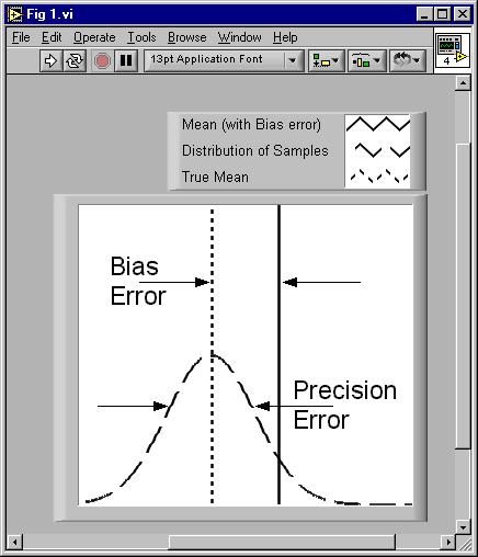
Figure 1, Errors in precision cause sample readings to spread out randomly from a sample mean. Accuracy (bias) errors are systematic, meaning that they impose a difference in the sample mean.

 A common measurement goal is to reduce measurement error, whatever the source. Reducing accuracy errors requires such initiatives as regularly scheduled calibration and choices regarding measurement design / setup. Improvements in this area often result from planning, diligence, and other “human” factors. Improving precision certainly entails these factors; in addition, its random nature means you can characterize it with statistical analysis.

 Any thorough discussion of statistical characterization of random fluctuations will dive into details related to statistical analysis, but I’ll refrain because such material resides in many textbooks. Instead, I’ll focus on some measurement-oriented specifics. Refs 2, 3 are a few helpful textbooks for background.

Precision dissection

With this measurement-oriented focus in mind, let’s return to the question “How precise is my measurement?” We’ll begin by considering a common measurement situation: given some data acquisition hardware, you want to sample the signal output of a transducer in order to measure a physical quantity associated with that transducer and you want to find the precision of your measurement. The situation might involve static measurements such as temperature measured with a RTD or thermocouple, or perhaps strain measured with a full- or half-bridge strain gauge. It might also involve dynamic signals, where the measurement of interest is a power spectrum or octave analysis.

 Because both static and dynamic signals are subject to random fluctuations, the following considerations apply for either class of signals. The difference between the two is often what you consider as a sample. For a static signal, a sample is often an instantaneous voltage level that you scale somehow to convert it to a physical quantity. For a dynamic signal, a sample could be an array of values that represents the power spectrum or octave analysis of a record of signal samples.

 Multiple samples (however you define them) are necessary to gauge your measurement precision. For one, remember that precision is actually a measure of random fluctuations that you won’t see if you are examining a single data point. Further, as discussed in a previous column (Ref 4), you should try to avoid using single samples as measurements. (Even in point-by-point control applications, where single-point measurements are common, there is often a hidden statistical treatment in the form of a filter—a mean value is a lowpass filter.)

Confidence in your measurement

Once you’ve acquired multiple samples, you can actually gauge precision with several powerful statistical analysis tools: confidence interval (CI) and confidence level (CL). The CI sets a range of values where you expect the mean of your measurements to reside. The CL is a percentage that specifies your statistical confidence as the probability of the mean falling in the CI. Fig 2 shows an example of a CI.

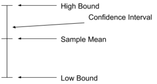
Figure 2, A confidence interval is a range of values delineated by numbers derived from a probability distribution (commonly a normal distribution or a T distribution) and a confidence level that you specify.

 In the context of CIs and CLs, it is common to refer to a population mean and not a sample mean. The difference is subtle, but important. The population mean represents the value that you would calculate with an infinite number of samples, while the sample mean is the arithmetic mean of your finite number of measurements. This distinction is what really imparts the practical benefit of working with CIs and CLs: they compensate for the fact that a direct measurement of a population mean isn’t possible because you cannot gather an infinite number of measurements.

 The practical use of these tools is to choose a desired CL and then use it, along with a set of measured values to determine a CI. Doing so is straightforward and is outlined in the steps below:

1. Verify that your data has a Normal (Gaussian) probability distribution. Making this assumption simplifies things, and is reasonable at least for a first pass—a famous mathematical theorem (Ref 5) relates that the mean value of an arbitrary signal is usually Gaussian. Nevertheless, statistical “goodness-of-fit” tools (Refs 1, 2) are available to allow you to empirically make this judgment.
2. Find the mean and standard deviation of your samples with the following formulas: and . For both equations, xi is a sample value and n is the number of samples. Modern programming environments, such as LabVIEW include ready-to-run functions to calculate these values.
3. Find the Standard Deviation of the means as
4. Choose a desired CL, and use it to find a corresponding area for 1-CL/2 under a Normal curve. LabVIEW includes a built-in function (VI) for this job: “Inv Normal Distribution.” (For smaller sample set sizes (a good rule of thumb is n<30), you can use the t-distribution as an alternative to the normal distribution. A corresponding LabVIEW function is “Inv T Distribution.”)
5. Multiply the resulting area under the normal curve by the standard deviation of the means, which you calculated in step 3. This value, along with the sample mean from step 2 defines the CI as , where z is the area from step 4.

 With these tools, your measurement evolves from a single value to a range of values and a probability. This extra information is useful in that the extent of the CI and the CL relate information about the number of measurements made and the random nature of the measurand. As shown in Fig 3, wider intervals at the same CL indicate fewer samples were used to gather the sample mean or an increased standard deviation.

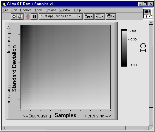
Figure 3, This intensity plot shows a general trend that appears in the width of a confidence interval (CI). The CI width decreases with an increasing number of samples or a decreasing Standard Deviation of your samples.

References

1. Smith, Steven W., A Scientist’s and Engineer’s Guide to Digital Signal Processing, California Technical Publishing, 1997, ISBN 0-9660176-3-3. The complete book is available online at http://www.dspguide.com.
2. Chugani, Mahesh, A. Samant, and M. Cerna, LabVIEW Signal Processing, Upper Saddle River: Prentice Hall PTR, 1998. ISBN 0-13-972449-4.
3. Beckwith, T, and R. Maragoni, Mechanical Measurements, 4ed., Reading: Addison-Wesley Pub Co., 1990. ISBN 0-201-17866-4.
4. Shearman, Sam, “Take Control of Noise with Spectral Averaging,” R&D Magazine’s Data Acquisition, Vol 4. No 7. July 2000, pgs 6-9.
5. Chung, Kai Lai, A Course on Probability Theory, 2ed, Academic Press, 2000. ISBN 0121741516

Sign in