Developing and Validating Simulation Models

This article will describe models for simulating the systems and controllers for the hardware emulation application described in Part 1 of the series.

• Part 1: Introduction
• Part 2: Ideal Model Examples
• Part 3: Sampled Data Aspects 
• Part 4: Engineering of Evaluation Hardware
• Part 5: Some FPGA Aspects

The engineering tools used will be the TI TINA Spice Simulator, MATLAB and Simulink.

The examples will be simple and for now, ideal continuous domain constructions.

An Example Arrangement for Simulation

Recall from article 1, the diagrams in Fig 1. showing a circuit on the LHS and a proposed emulation scheme on the RHS. As noted before, this is not necessarily the best practical arrangement and it is also not the only topology available.

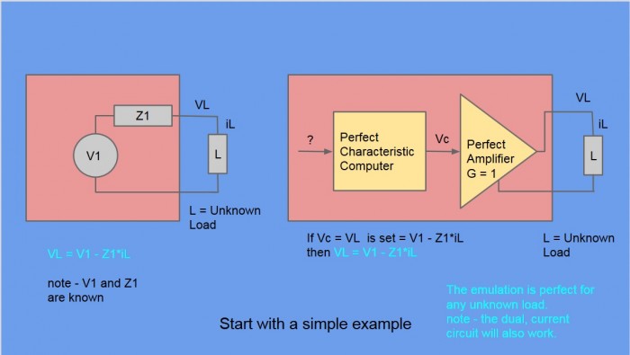
Fig 1. One of several equivalent topologies for hardware emulation

We are proposing that in an ideal case, the example circuit on the LHS can be emulated by means of a perfect amplifier, a current measurement applied to a characteristic impedance Z1 and a summer combining the voltage on the Z1 impedance and a Voltage V1.

Spice Simulations 

I use LinearTech(ADI) LTSpice and TI TINA Spice equally for circuit simulation, but in this article, TI TINA will be used. 

Circuit Sourcing Case

Fig 2 Shows the circuit and arrangement for a specific example of Fig 1. Apologies for the small differences in component labelling.

The Reference circuit is a Voltage VG1 and a source impedance Z1 of 100ohms + (300ohms//100nF). The Load is a 400 ohm resistor. The emulation arrangement is as previously described and we wish to verify that the circuit characteristic (Bode Plot) is the same for both cases.

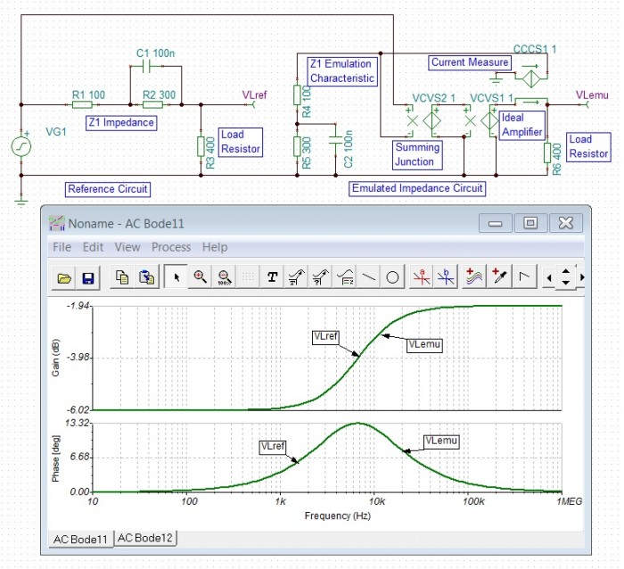
Fig 2. Spice simulation and Bode plot of Reference and Emulation Circuits - Circuit Sourcing

As can be seen in the plots, the two circuit responses are coincident, as required.

Circuit Sinking Case

Fig 3 Shows the corresponding case where the Load side has the voltage generator and the circuit is sinking current rather than sourcing it.

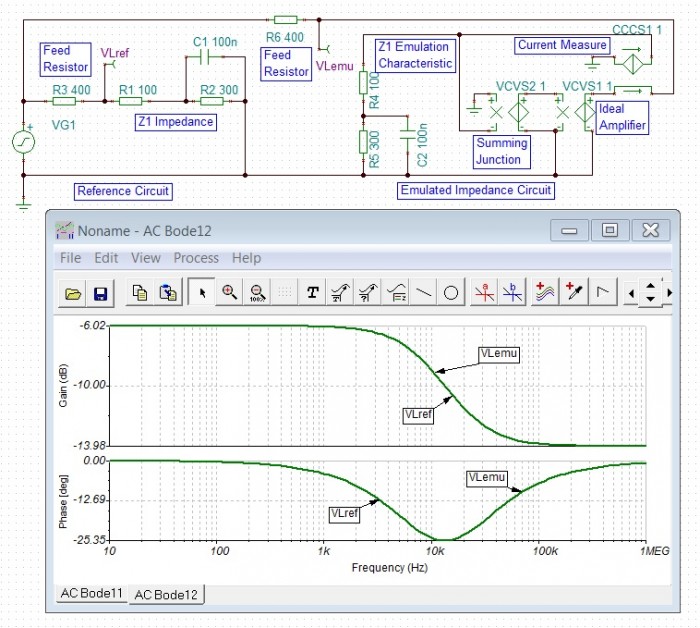
Fig 3. Current Sinking case

Again, the two circuit responses are coincident, as required.

Discussion

So, we have developed a scheme to replace an example circuit of 2 resistors, a capacitor and a voltage source by 2 resistors, a capacitor, a voltage source, an amplifier, a summer and a current measurement. That needs a bit of justification.

1.  In a real commercial application, the required circuits included precision, selectable, large-value Inductors and Capacitors and selectable Resistors all operating at several hundred volts and currents up to 150mA. These are very expensive and physically large components. By making use of a specialist amplifier such as this one from Apex, we could with the help of some scaling and gain use a selection of small signal R,L & Cs instead of the prohibitively expensive passive only solution. But, the real end-game is ....
2. As per the title of this article, the aim is to generate complex circuit emulation characteristics with code. In a previous project this was done in C on an ADI Sharc DSP. Now, we are looking at what can be achieved by a Floating-Point centric FPGA. 

MATLAB Simulations 

The following MATLAB code simulates and plots the circuit response for both circuit sourcing (VLrefa) and circuit sinking(VLrefb) reference circuits.

opts = bodeoptions('cstprefs');  
opts.FreqUnits = 'Hz';          % change the bode options to Hz
s = tf('s');                    % declare the s operator
R1 = 100;                       % Series Part of Z1
R2 = 300;                       % Parallel Resistive Part of Z1
C  = 100e-9;                    % Parallel Capacitive Part of Z1
RL = 400;                       % Load/Feed Resistor
Z1Para = 1/((1/R2) + ( C*s)) ;                    % Parallel Part of Z1
altZ1Para = ( R2* (1/(C*s)))/ ( R2 + (1/(C*s))) ; % Parallel Part of Z1
Z1 = R1 + Z1Para;                 % Reference impedance for emulation  
VLrefa = RL / ( RL + Z1 );        % Potential divider equation for voltage 
                                  % when Z1 is driving RL
VLrefb = Z1 / ( RL + Z1 );        % Potential divider equation for voltage 
                                  % when RL is driving Z1 
bodeplot(VLrefa,VLrefb,{1,10000000},opts) % show VL
grid on                                   % grid on

Which results in the following circuit plots in Fig 4.

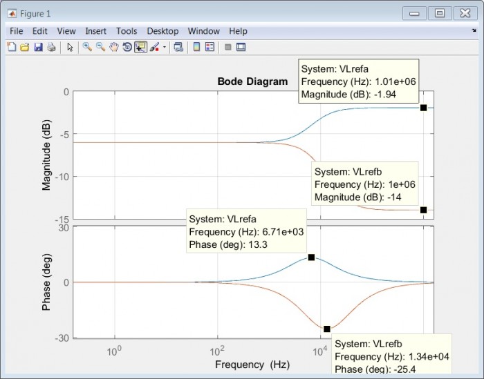
Fig 4. MATLAB Plots of the reference circuit for both sourcing(VLrefa) and sinking(VLrefb) conditions

These graphs correspond to the Spice circuit responses shown in Fig 2 and Fig 3.

Discussion

These MATLAB plots are only showing the simple passive reference circuit responses, the construction of the emulation schemes will be done in Simulink and compared to the MATLAB references.

One quirk ? in MATLAB was noticed in the calculation of parallel components. For two parallel components we can opt for either a) 1/(sum of inverses) or b) the product/sum equations as per the code.

Z1Para = 1/((1/R2) + ( C*s)) ;                    % Parallel Part of Z1
altZ1Para = ( R2* (1/(C*s)))/ ( R2 + (1/(C*s))) ; % Parallel Part of Z1

When MATLAB reports these we get :-

a) Z1Para     = 1/(1e-07 s + 0.003333) and

b) altZ1Para = 3e-05 s/(3e-12 s^2 + 1e-07 s)

Calculation b) is equivalent to calculation a), but is overcomplicated by an extra s top and bottom, which can cancel out.

We therefore stick to the sum of inverses method.

Simulink Simulations 

At this time, I am using MATLAB to interact with Simulink models to get the best of both tools.

As many of you will know you don't simply get a Bode Plot from Simulink. There is an averaging spectrum analyser block that might be useful and also a tool in one of the tool boxes I don't have. So, I rolled my own Simulink Bode plotter using IQ extraction of the excitation frequency in the time domain. This will be very useful when the simulations include sampled data controllers.

The Bode plotter will not be documented, as it is rather a slow, inefficient tool at the moment.

Note - It is noted that the Simulink block diagrams below, contain algebraic loops which generate warnings. However, the solver seems quite capable of resolving them so for now we will let it run without further attention.

Circuit Sourcing Case

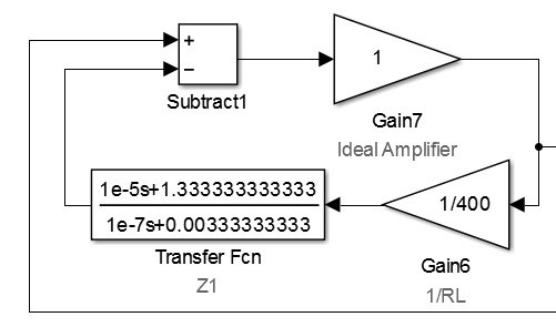
Fig 5. Simulink Model of the Example Emulation Arrangement - Sourcing Case

As per previous description

"We are proposing that in an ideal case, the example circuit on the LHS can be emulated by means of a perfect amplifier, a current measurement applied to a characteristic impedance Z1 and a summer (with 1 i/p negative) combining the voltage on the Z1 impedance and a Voltage V1. "

Here, VL is the voltage output from the Ideal Amplifier and the current is "measured" by  Gain6 = 1/RL, which is then applied to impedance to be emulated Z1. The summer drives the Ideal Amplifier from Voltage output of Z1 - the driving signal V1 applied to the subtracter.

Fig 6 shows the Reference MATLAB Bode response and the Simulink Bode response.

Fig 6. MATLAB reference and Simulink emulation plots - Sourcing case.

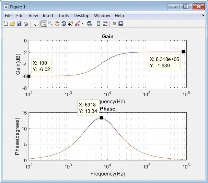
These are in close agreement with the previous MATLAB results, as they should be given that the MATLAB transfer function is the same as used before.

Circuit Sinking Case

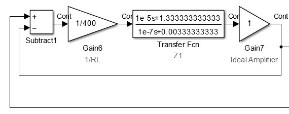
Fig 7. Simulink Model of the Example Emulation Arrangement - Sinking Case

This is just a small re-arrangement to the Sourcing Case, to move the applied voltage to the resistor.

Fig 8 shows the Reference MATLAB Bode response and the Simulink Bode response.

Fig 8. MATLAB reference and Simulink emulation plots - Sinking case.

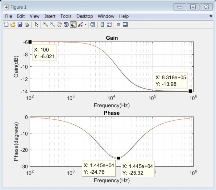
The granularity of frequency points is rather coarse to reduce the simulation time, so comparison with MATLAB only or Spice responses is not exact. However, there is a noticeable difference of 0.56 degrees phase, between the MATLAB value -25.32 and the Simulink value -24.76. at the same frequency. This maybe due to Simulink accuracies vs MATLAB accuracies given that MATLAB is just evaluating an expression in s where as Simulink is simulating a closed-loop time domain response and then performing some modestly complicated sums to extract input and output magnitude and phase.

In any case the divergence is small in the scale of things and may be re-visited later.

Discussion

Simulations of reference and emulation circuits have been developed in Spice, MATLAB and Simulink environments. 

A MATLAB driven Simulink approach appears to offer a good combination of power, flexibility and ease of understanding for the detailed work to come.

The small differences apparent between the MATLAB reference results and the Simulink Emulation results may warrant further investigation, but for now the techniques are fine for general development.

Coming Next .....

  Next up will be a look at some sampled-data aspects.

Sign in